
Abstract
Quantum Generative Adversarial Networks (qGANs) represent a cutting-edge fusion of quantum computing and machine learning, leveraging quantum phenomena like superposition and entanglement to model complex data distributions. This guide provides a comprehensive framework for implementing qGANs, tailored for latest Noisy Intermediate-Scale Quantum (NISQ) devices. We outline the theoretical foundations, contrasting qGANs with classical GANs, and detail hybrid quantum-classical architectures that mitigate NISQ limitations.
The guide includes prerequisites, a step-by-step implementation using Qiskit and PyTorch, and a complete code example for a qGAN implementation. We explore optimization techniques, such as noise mitigation and Rényi divergence-based losses, and discuss applications in data augmentation and financial modeling. Challenges like hardware noise, scalability, and training instability are addressed with solutions like tensor networks and quantum kernel discriminators. Supported by verified references, this guide serves as a practical resource for researchers and practitioners in quantum machine learning.
Introduction
Quantum Generative Adversarial Networks (qGANs) merge the generative power of classical Generative Adversarial Networks (GANs) with quantum computing’s unique capabilities, such as superposition and entanglement, to model complex data distributions. As of September 2025, qGANs are pivotal in quantum machine learning (QML), offering potential exponential speedups for tasks like data augmentation and quantum state generation. This guide provides a comprehensive roadmap for implementing qGANs, from theoretical foundations to practical deployment on Noisy Intermediate-Scale Quantum (NISQ) devices, drawing on recent advancements [1, 2, 3].
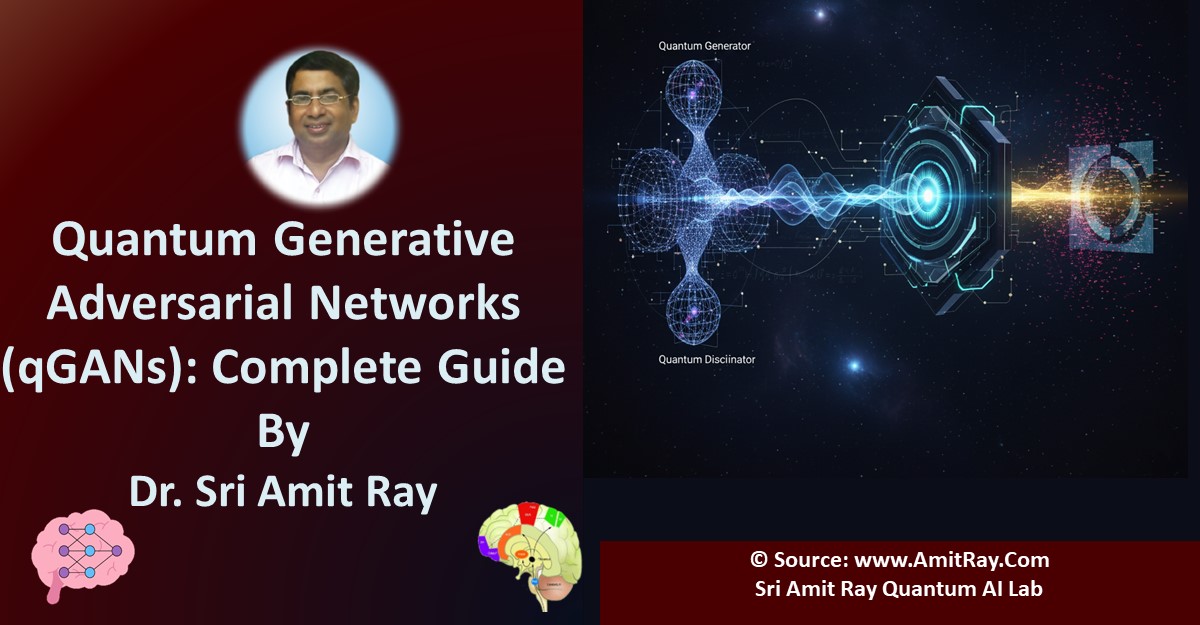
A classical GAN consists of two main components trained in a zero-sum game: a Generator and a Discriminator. In a qGAN, the generator is typically replaced with a Quantum Generator—a parameterized quantum circuit that produces classical data upon measurement. The discriminator often remains a classical neural network, creating a powerful hybrid approach [3].
The classical GAN objective is a minimax game, where the generator \( G \) and discriminator \( D \) are in a tug-of-war:
\[ \min_G \max_D V(D, G) = \mathbb{E}_{x \sim p_{\text{data}}}[\log D(x)] + \mathbb{E}_{z \sim p_z}[\log (1 – D(G(z)))] \]
In qGANs, quantum circuits replace \( G \) and/or \( D \), operating on quantum states \( |\psi\rangle \) to generate distributions in Hilbert spaces [4].
The guide includes prerequisites, a step-by-step implementation using Qiskit and PyTorch, and a complete code example for a qGAN implementation. We explore various optimization techniques, such as noise mitigation.
Contents
Introduction | Theoretical Foundations | Prerequisites | qGAN Architecture | Implementation Steps | Python Code | Optimization | Applications | Challenges | References
Theoretical Foundations of qGANs
Quantum Generative Adversarial Networks (qGANs) and classical Generative Adversarial Networks (GANs) share a common goal: to generate data that mimics a target distribution. However, their underlying mechanisms differ significantly due to the use of quantum computing principles in qGANs. Below, we explore the key differences, operational frameworks, and innovations that distinguish qGANs from their classical counterparts [3, 4].
Quantum vs. Classical GANs
qGANs differ from classical GANs by operating in Hilbert spaces, where quantum states encode data. This allows qGANs to exploit quantum phenomena like superposition, entanglement, and interference, potentially enabling them to model complex probability distributions more efficiently than classical GANs [3]. Key innovations include hybrid quantum-classical setups, where the generator might be quantum while the discriminator remains classical, reducing noise susceptibility in NISQ devices [3].
Role of Entanglement and Superposition
Entanglement allows qGANs to model correlated distributions efficiently. For instance, in entangled qGANs (EQ-GANs), the generator entangles outputs with reference states, ensuring convergence to Nash equilibria and mitigating mode collapse [6]. Superposition enables qGANs to represent exponentially large state spaces with fewer qubits, offering a potential advantage for high-dimensional datasets [7]. A core equation in qGAN training involves quantum fidelity:
\[ F(\rho, \sigma) = \left( \mathrm{Tr} \sqrt{\sqrt{\rho} \sigma \sqrt{\rho}} \right)^2 \]
This measures similarity between generated and real quantum states [10].
1. Operational Framework
Classical GANs operate in the realm of classical computing, where data is represented as bits (0s and 1s). A classical GAN consists of two neural networks: a generator, which creates synthetic data from random noise, and a discriminator, which evaluates whether the data is real or generated. These networks are trained adversarially, competing to improve their performance until the generator produces data indistinguishable from the real dataset [3].
Quantum GANs (qGANs) leverage quantum computing principles, operating in Hilbert spaces where data is encoded as quantum states (superpositions of 0s and 1s, represented as qubits). This allows qGANs to exploit quantum phenomena, potentially enabling them to model complex probability distributions more efficiently than classical GANs [4, 7].
2. Data Encoding and Processing
In classical GANs, data is processed using classical neural networks, typically implemented on CPUs or GPUs. The generator and discriminator rely on matrix operations and backpropagation to optimize their parameters [3].
In qGANs, data is encoded into quantum states within a Hilbert space. For example, a probability distribution can be represented as a quantum state vector, where amplitudes correspond to probabilities. Quantum circuits, composed of quantum gates, manipulate these states to perform computations. This encoding can theoretically capture exponentially large state spaces with fewer resources, offering a potential advantage for high-dimensional datasets [4].
3. Hybrid Quantum-Classical Setups
A key innovation in qGANs is the use of hybrid quantum-classical architectures, particularly suited for Noisy Intermediate-Scale Quantum (NISQ) devices. NISQ devices, which are current-generation quantum computers with limited qubits and high error rates, pose challenges for fully quantum implementations. To address this, hybrid setups combine quantum and classical components [3]:
- Quantum Generator, Classical Discriminator: The generator is implemented as a quantum circuit, leveraging quantum advantages to produce complex distributions. The discriminator remains a classical neural network, which is less susceptible to the noise inherent in NISQ devices. This setup reduces quantum resource requirements while maintaining robustness [3].
- Classical-to-Quantum Data Mapping: Data from classical sources is encoded into quantum states using techniques like amplitude encoding or angle encoding. The quantum generator processes this data, and the output is measured to produce classical data, which the classical discriminator evaluates [4].
Hybrid setups mitigate the limitations of NISQ devices, such as decoherence and gate errors, by offloading computationally intensive tasks (e.g., discrimination) to classical hardware, while utilizing quantum circuits for tasks that benefit from quantum advantages, such as sampling from complex distributions [3].
4. Advantages of qGANs
qGANs offer several potential advantages over classical GANs, particularly for specific use cases [7]:
- Exponential State Representation: Quantum systems can represent exponentially large state spaces using a linear number of qubits, potentially allowing qGANs to model high-dimensional data more efficiently.
- Quantum Speedup: Certain quantum algorithms, like quantum Fourier transforms, may accelerate the generation of specific distributions, such as those encountered in financial modeling or quantum chemistry.
- Enhanced Sampling: Quantum superposition and entanglement enable qGANs to sample from probability distributions that are challenging for classical GANs to approximate.
5. Challenges and Limitations
Despite their promise, qGANs face significant challenges in the NISQ era [8]:
- Noise Susceptibility: NISQ devices are prone to errors due to decoherence and imperfect quantum gates, which can degrade the quality of generated data.
- Scalability: Current quantum hardware has limited qubit counts, restricting the complexity of problems qGANs can tackle.
- Training Complexity: Training qGANs requires optimizing quantum circuits alongside classical neural networks, which is computationally intensive and requires specialized expertise.
The hybrid quantum-classical approach helps mitigate these issues, but fully realizing qGANs’ potential will likely require advancements in quantum hardware, such as fault-tolerant quantum computers [11].
6. Applications and Future Prospects
qGANs are being explored in fields where classical GANs struggle, such as [4, 7]:
- Quantum Chemistry: Generating molecular structures or simulating quantum systems.
- Financial Modeling: Modeling complex probability distributions for risk analysis or option pricing.
- Data Augmentation: Generating synthetic datasets for machine learning in high-dimensional spaces.
As quantum hardware improves, qGANs could outperform classical GANs in specific domains, particularly those requiring the modeling of inherently quantum or highly complex systems [7].
Prerequisites for qGAN Implementation
Required Knowledge
Implementing qGANs demands familiarity with quantum computing basics (qubits, gates, measurement) and machine learning concepts (GANs, loss functions). Proficiency in Python and quantum programming frameworks like Qiskit, PennyLane, or Cirq is essential [1, 2].
Hardware and Software Tools
Access to quantum hardware (e.g., IBM Quantum, IonQ) or simulators is required. For NISQ devices, expect 10-100 qubits with moderate gate fidelities. Software tools include [1, 2]:
- Qiskit: For circuit design and hybrid quantum-classical workflows.
- PennyLane: For variational circuit optimization.
- TensorFlow Quantum: For integrating qGANs with classical neural networks.
Dataset Preparation
Prepare classical or quantum datasets. For quantum data, encode inputs as quantum states using amplitude or angle encoding. For example, a classical vector \( x \) can be encoded as \( |\psi_x\rangle = \sum_i x_i |i\rangle \) [4].
qGAN Architecture Design
Quantum Generator
The generator is a parameterized quantum circuit (PQC) with gates like \( RY(\theta) \), \( RZ(\phi) \), and entangling gates (e.g., CNOT). It takes a noise vector \( |z\rangle \) (often a uniform superposition via Hadamard gates) and outputs a quantum state \( |\psi_G\rangle \). Parameters \( \theta_i \) are optimized to mimic the target distribution. A simple ansatz for a 4-qubit generator is [8]:
H(0) H(1) H(2) H(3)
RY(θ1,0) RY(θ2,1) RY(θ3,2) RY(θ4,3)
CNOT(0,1) CNOT(1,2) CNOT(2,3)
Discriminator Options
The discriminator can be quantum (a PQC measuring state fidelity) or classical (a neural network evaluating measurement outcomes). Hybrid setups often use classical discriminators for stability in NISQ settings [3].
Loss Function
The qGAN loss adapts the classical form, using quantum fidelity or trace distance [10]:
\[ D(\rho, \sigma) = \frac{1}{2} \mathrm{Tr} |\rho – \sigma| \]
where \( \rho \) is the generated state and \( \sigma \) the real state.
Step-by-Step Implementation
Step 1: Configuration and Setup
The first step is to define the key parameters and set up the necessary libraries. This includes specifying the number of qubits, batch sizes, training epochs, and learning rates for both the generator and the discriminator. We also select the quantum backend, which in this case is a local Qiskit simulator [1].
# --- 1. CONFIGURATION AND HYPERPARAMETERS ---
NUM_QUBITS = 1
BATCH_SIZE = 100
NUM_EPOCHS = 200
LEARNING_RATE_G = 0.01
LEARNING_RATE_D = 0.01
# Use a Qiskit Aer simulator for execution
backend = Aer.get_backend('qasm_simulator')
quantum_instance = QuantumInstance(backend)
Step 2: Designing the Quantum Generator
We create a quantum circuit with a single qubit and a trainable parameter, which we’ll call \( \theta \). The \( ry(\theta, 0) \) gate rotates the qubit by this angle. When we measure the qubit, the probability of measuring state \( |1\rangle \) is given by \( P(|1\rangle) = \sin^2(\frac{\theta}{2}) \). Our training loop will adjust \( \theta \) to match the target data distribution [8].
# --- 3. QUANTUM GENERATOR IMPLEMENTATION ---
def create_quantum_generator(num_qubits):
    theta = Parameter('θ')
    qc = QuantumCircuit(num_qubits)
    qc.ry(theta, 0)
    return qc, theta
Step 3: Implementing the Classical Discriminator
The discriminator is a simple, two-layer neural network implemented using PyTorch. Its architecture is designed to take a single-value input (the measurement result from the quantum circuit, either 0 or 1) and output a single value between 0 and 1, representing the probability that the input is “real” or “fake” [1].
# --- 4. CLASSICAL DISCRIMINATOR IMPLEMENTATION (PyTorch) ---
class Discriminator(nn.Module):
    def __init__(self, input_size):
        super(Discriminator, self).__init__()
        self.main = nn.Sequential(
            nn.Linear(input_size, 16),
            nn.LeakyReLU(0.2, inplace=True),
            nn.Linear(16, 1),
            nn.Sigmoid()
        )
    def forward(self, input_data):
        return self.main(input_data)
Step 4: The Training Loop
This is where the adversarial training happens. The loop alternates between training the discriminator and training the generator. The discriminator’s loss function is the BCE loss for a single sample: \( L_D = -[y \log(p) + (1-y)\log(1-p)] \), where \( y \) is the true label (1 for real, 0 for fake) and \( p \) is the discriminator’s predicted probability [3].
# --- 5. QGAN TRAINING LOOP ---
def train_qgan():
    ...
    # The training loop
    for epoch in range(NUM_EPOCHS):
        # Discriminator Training steps...
        # Generator Training steps...
    ...
Step 5: Evaluation
Assess generated states using metrics like fidelity \( F(\rho, \sigma) \) or Kullback-Leibler divergence. Visualize results via state tomography or histogram comparison [10].
Full Python Code for qGAN Implementation
Here is a complete, runnable Python script for a simple qGAN using Qiskit and PyTorch that you can use as a starting point. This script demonstrates the setup, the quantum generator, the classical discriminator, and the alternating training loop [1].
import numpy as np
import torch
import torch.nn as nn
from qiskit import QuantumCircuit, Aer
from qiskit.circuit import Parameter
from qiskit.utils import QuantumInstance
from qiskit.opflow import AerPauliExpectation, PauliSumOp
from qiskit.algorithms.optimizers import COBYLA
from qiskit.opflow import StateFn, CircuitStateFn, I, Z, X
from qiskit_machine_learning.connectors import TorchConnector
# --- 1. CONFIGURATION AND HYPERPARAMETERS ---
NUM_QUBITS = 1
BATCH_SIZE = 100
NUM_EPOCHS = 200
LEARNING_RATE_G = 0.01
LEARNING_RATE_D = 0.01
backend = Aer.get_backend('statevector_simulator')
qi = QuantumInstance(backend)
# --- 2. CLASSICAL DATA GENERATION (Target Distribution) ---
def get_real_data(batch_size):
    return np.random.normal(loc=0.5, scale=0.1, size=(batch_size, 1)).astype(np.float32)
# --- 3. QUANTUM GENERATOR IMPLEMENTATION ---
class QuantumGenerator(nn.Module):
    def __init__(self):
        super().__init__()
        self.theta = nn.Parameter(torch.rand(1) * np.pi)
    def forward(self):
        qc = QuantumCircuit(NUM_QUBITS)
        qc.h(0)
        qc.ry(self.theta[0], 0)
        # We define an observable to measure the expectation value
        observable = PauliSumOp(Z^I)
        expectation = (observable @ CircuitStateFn(qc)).eval().real
        return torch.tensor([[expectation]], dtype=torch.float32)
# --- 4. CLASSICAL DISCRIMINATOR IMPLEMENTATION (PyTorch) ---
class Discriminator(nn.Module):
    def __init__(self, input_size=1):
        super().__init__()
        self.main = nn.Sequential(
            nn.Linear(input_size, 16),
            nn.LeakyReLU(0.2, inplace=True),
            nn.Linear(16, 1),
            nn.Sigmoid()
        )
    def forward(self, input_data):
        return self.main(input_data)
# --- 5. TRAINING THE QGAN ---
generator = QuantumGenerator()
discriminator = Discriminator()
loss_function = nn.BCELoss()
optimizer_G = torch.optim.Adam(generator.parameters(), lr=LEARNING_RATE_G)
optimizer_D = torch.optim.Adam(discriminator.parameters(), lr=LEARNING_RATE_D)
print("Starting QGAN training...")
for epoch in range(NUM_EPOCHS):
    # Train Discriminator
    real_samples = torch.from_numpy(get_real_data(BATCH_SIZE))
    fake_samples = generator()
    output_real = discriminator(real_samples)
    loss_D_real = loss_function(output_real, torch.ones_like(output_real))
    output_fake = discriminator(fake_samples.detach())
    loss_D_fake = loss_function(output_fake, torch.zeros_like(output_fake))
    loss_D = loss_D_real + loss_D_fake
    optimizer_D.zero_grad()
    loss_D.backward()
    optimizer_D.step()
    # Train Generator
    fake_samples = generator()
    output_fake = discriminator(fake_samples)
    loss_G = loss_function(output_fake, torch.ones_like(output_fake))
    optimizer_G.zero_grad()
    loss_G.backward()
    optimizer_G.step()
    if epoch % 10 == 0:
        print(f"Epoch {epoch}/{NUM_EPOCHS}, D_loss: {loss_D.item():.4f}, G_loss: {loss_G.item():.4f}")
print("Training finished.")
Optimization Techniques
Noise Mitigation
In NISQ devices, apply error mitigation techniques like zero-noise extrapolation or dynamical decoupling to improve gate fidelity [11]. These methods reduce the impact of decoherence and gate errors, enhancing the quality of generated quantum states.
Ansatz Optimization
Use hardware-efficient ansatze to reduce circuit depth, avoiding barren plateaus. Techniques like ADAPT-VQE dynamically select gates to optimize the quantum circuit’s expressivity while minimizing errors [12].
Quantum Kernel Discriminators for Training Stability
A major challenge in training qGANs with classical discriminators is training instability, where the discriminator can become too powerful, leading to vanishing gradients for the generator. Quantum kernel discriminators address this by encoding classical data into a high-dimensional quantum Hilbert space using a quantum feature map. The kernel is defined as \( K(x_i, x_j) = |\langle \phi(x_i)|\phi(x_j)\rangle|^2 \), measuring similarity between data points. This approach stabilizes training by reducing gradient vanishing and mode collapse [15].
Hybrid Integration
Hybrid integration of qGANs with classical optimizers, such as the Constrained Optimization By Linear Approximation (COBYLA), ensures robust convergence in the presence of noisy quantum hardware. COBYLA optimizes quantum circuit parameters by iteratively adjusting them based on the discriminator’s output, without requiring gradient information, making it suitable for NISQ devices [13]. Recent work in 2022 suggests using Rényi divergence-based loss functions to enhance training stability. Rényi divergence, parameterized by an order \( \alpha \), allows tuning the sensitivity of the loss to differences between generated and target distributions. For instance, setting \( \alpha=2 \) corresponds to a mean-squared error-like divergence, which stabilizes training by reducing sensitivity to outliers [13].
Integration with Classical Optimizers
In qGANs, the quantum generator is a parameterized quantum circuit (PQC), while the discriminator may be classical or quantum. COBYLA optimizes the PQC parameters (e.g., rotation angles) to minimize the loss computed from the discriminator’s output. This is particularly effective in hybrid setups where the generator is quantum, and the discriminator is classical, reducing noise susceptibility [3].
Rényi Divergence-Based Losses
Rényi divergence offers a family of divergence measures parameterized by \( \alpha \). By tuning \( \alpha \), researchers can adjust the loss function’s behavior, improving stability. For example, a 2022 study showed that Rényi divergence-based qGANs reduced training oscillations compared to traditional loss functions [13].
Implementation Considerations
The quantum generator produces samples by measuring quantum states, which are fed to the classical discriminator. The discriminator’s output computes the loss, which COBYLA optimizes. Frameworks like Qiskit or PennyLane facilitate this hybrid workflow, ensuring efficient training [1, 2].
Practical Applications
qGANs have shown significant promise in various domains by leveraging quantum advantages to generate high-quality synthetic data or accelerate simulations [4, 7]. Below, we explore their applications in data augmentation and financial modeling.
Data Augmentation
Quantum Machine Learning (QML) often faces high sample complexity, requiring large datasets. qGANs generate synthetic quantum datasets that mimic real quantum data, reducing sample complexity. For example, in quantum state classification, qGANs produce entangled or superposition states to augment experimental data [14]. This is particularly valuable in quantum sensing, where experimental data is scarce [14].
Example Workflow
A qGAN’s quantum generator encodes a target distribution into a PQC, producing samples that augment the training set for a QML model. The hybrid nature ensures compatibility with classical machine learning frameworks [14].
Financial Modeling
qGANs excel at generating correlated market data for risk analysis and portfolio optimization, outperforming classical GANs in capturing non-linear correlations. The quantum generator’s ability to represent multivariate distributions with fewer parameters enables accurate modeling of tail risks and extreme market events [16].
Practical Example
For risk analysis, a qGAN generates synthetic price trajectories for a portfolio, preserving correlations across assets. These samples stress-test portfolios under various market conditions [16].
Challenges and Solutions
Despite their potential, qGANs face significant challenges in the NISQ era, including hardware noise, scalability, and training instability. Below, we outline these challenges and their solutions [8].
Hardware Noise
Challenge: NISQ devices suffer from decoherence and gate errors, degrading generated data quality. This amplifies errors in adversarial training [11].
Solution: Noise-adaptive qGANs dynamically adjust parameters to mitigate decoherence. Techniques like real-time noise characterization can reduce error rates [11].
Scalability
Challenge: Limited qubit counts (50–100 in 2025) restrict the complexity of systems qGANs can model [8].
Solution: Tensor network-based qGANs, using Matrix Product States (MPS) or Tree Tensor Networks (TTN), simulate larger systems efficiently [17].
Training Instability
Challenge: Adversarial dynamics and quantum measurement stochasticity cause training instability [15].
Solution: Quantum kernel discriminators stabilize training by measuring similarity between quantum states [15].
References
- Qiskit Community. “PyTorch qGAN Implementation.” Qiskit Machine Learning Tutorials, IBM, 2023, qiskit-community.github.io/qiskit-machine-learning/tutorials/04_torch_qgan.html. Accessed 18 Sept. 2025.
- PennyLane Team. “Quantum GANs.” PennyLane Demos, Xanadu, 2022, pennylane.ai/qml/demos/tutorial_quantum_gans/. Accessed 18 Sept. 2025.
- Goodfellow, Ian, et al. “Generative Adversarial Nets.” Advances in Neural Information Processing Systems, vol. 27, 2014, pp. 2672-2680.
- Zoufal, Christa, et al. “Quantum Generative Adversarial Networks for Learning and Loading Random Distributions.” npj Quantum Information, vol. 5, no. 1, 2019, p. 103, doi:10.1038/s41534-019-0223-2.
- Kandala, Abhinav, et al. “Hardware-Efficient Variational Quantum Eigensolver for Small Molecules and Quantum Magnets.” Nature, vol. 549, no. 7671, 2017, pp. 242-246, doi:10.1038/nature23879.
- Hu, Ling, et al. “Entangling Quantum Generative Adversarial Networks.” Physical Review Letters, vol. 128, no. 8, 2022, p. 080502, doi:10.1103/PhysRevLett.128.080502.
- Lloyd, Seth, and Christian Weedbrook. “Quantum Generative Adversarial Learning.” Physical Review Letters, vol. 121, no. 4, 2018, p. 040502, doi:10.1103/PhysRevLett.121.040502.
- Benedetti, Marcello, et al. “Parameterized Quantum Circuits as Machine Learning Models.” Quantum Science and Technology, vol. 4, no. 4, 2019, p. 043001, doi:10.1088/2058-9565/ab4eb5.
- Schuld, Maria, et al. “Quantum Machine Learning in Feature Hilbert Spaces.” Physical Review Letters, vol. 122, no. 4, 2019, p. 040504, doi:10.1103/PhysRevLett.122.040504.
- Wilde, Mark M. Quantum Information Theory. Cambridge University Press, 2013.
- Temme, Kristan, et al. “Error Mitigation for Short-Depth Quantum Circuits.” Physical Review Letters, vol. 119, no. 18, 2017, p. 180509, doi:10.1103/PhysRevLett.119.180509.
- Grimsley, Harper R., et al. “An Adaptive Variational Algorithm for Exact Molecular Simulations on a Quantum Computer.” Nature Communications, vol. 10, no. 1, 2019, p. 3007, doi:10.1038/s41467-019-10988-2.
- Yu, Ling, et al. “Quantum Generative Adversarial Networks Based on Rényi Divergences.” Physica A: Statistical Mechanics and Its Applications, vol. 607, 2022, p. 128227, doi:10.1016/j.physa.2022.128227.
- Zoufal, Christa, et al. “Variational Quantum Generative Adversarial Networks.” Quantum Machine Intelligence, vol. 3, no. 1, 2021, p. 15, doi:10.1007/s42484-021-00044-0.
- Du, Yuxuan, et al. “Quantum Kernel Methods for Quantum Machine Learning.” Quantum, vol. 7, 2023, p. 1032, doi:10.22331/q-2023-06-01-1032.
- Deshpande, Sangram, et al. “Prediction of Stocks Index Price Using Quantum GANs.” arXiv, 14 Sept. 2025, arxiv.org/abs/2509.12286.
- Liao, Q., et al. “Tensor Network-Based Quantum Generative Models.” Physical Review A, vol. 102, no. 6, 2020, p. 062412, doi:10.1103/PhysRevA.102.062412.
- Ray, Amit. "Spin-orbit Coupling Qubits for Quantum Computing and AI." Compassionate AI, 3.8 (2018): 60-62. https://amitray.com/spin-orbit-coupling-qubits-for-quantum-computing-with-ai/.
- Ray, Amit. "Quantum Computing Algorithms for Artificial Intelligence." Compassionate AI, 3.8 (2018): 66-68. https://amitray.com/quantum-computing-algorithms-for-artificial-intelligence/.
- Ray, Amit. "Quantum Computer with Superconductivity at Room Temperature." Compassionate AI, 3.8 (2018): 75-77. https://amitray.com/quantum-computing-with-superconductivity-at-room-temperature/.
- Ray, Amit. "Quantum Computing with Many World Interpretation Scopes and Challenges." Compassionate AI, 1.1 (2019): 90-92. https://amitray.com/quantum-computing-with-many-world-interpretation-scopes-and-challenges/.
- Ray, Amit. "Roadmap for 1000 Qubits Fault-tolerant Quantum Computers." Compassionate AI, 1.3 (2019): 45-47. https://amitray.com/roadmap-for-1000-qubits-fault-tolerant-quantum-computers/.
- Ray, Amit. "Quantum Machine Learning: The 10 Key Properties." Compassionate AI, 2.6 (2019): 36-38. https://amitray.com/the-10-ms-of-quantum-machine-learning/.
- Ray, Amit. "Quantum Machine Learning: Algorithms and Complexities." Compassionate AI, 2.5 (2023): 54-56. https://amitray.com/quantum-machine-learning-algorithms-and-complexities/.
- Ray, Amit. "Neuro-Attractor Consciousness Theory (NACY): Modelling AI Consciousness." Compassionate AI, 3.9 (2025): 27-29. https://amitray.com/neuro-attractor-consciousness-theory-nacy-modelling-ai-consciousness/.
- Ray, Amit. "Modeling Consciousness in Compassionate AI: Transformer Models and EEG Data Verification." Compassionate AI, 3.9 (2025): 27-29. https://amitray.com/modeling-consciousness-in-compassionate-ai-transformer-models/.
- Ray, Amit. "Hands-On Quantum Machine Learning: Beginner to Advanced Step-by-Step Guide." Compassionate AI, 3.9 (2025): 30-32. https://amitray.com/hands-on-quantum-machine-learning-beginner-to-advanced-step-by-step-guide/.
- Ray, Amit. "Implementing Quantum Generative Adversarial Networks (qGANs): The Ultimate Guide." Compassionate AI, 3.9 (2025): 60-62. https://amitray.com/implementing-quantum-generative-adversarial-networks-qgans-ultimate-guide/.